Getting started: your first simulation
A 90° silicon waveguide bend, simulated by
examples/waveguide_bend.py: a
transmission value, a field image, and the result open in the viewer. Install bifrost first, and run
the script on a GPU if you have one.
The device is a 500 nm wide, 220 nm thick silicon strip in silica: gdsfactory's bend_circular cell, a 5 µm radius
arc, with both ports extended straight to the edge of the simulation box. TE0 light at 1.55 µm is launched into the
extension of port o1, and the script measures how much of it leaves port o2 in TE0.
Run it
Save the complete script as waveguide_bend.py and run it:
Output on an NVIDIA L40S (yours will differ slightly):
transmission: 1.0008
wall time:    32.4 s (compilation included)
peak memory:  1.2 GiB on cuda:0
field image:  waveguide_bend_field.png
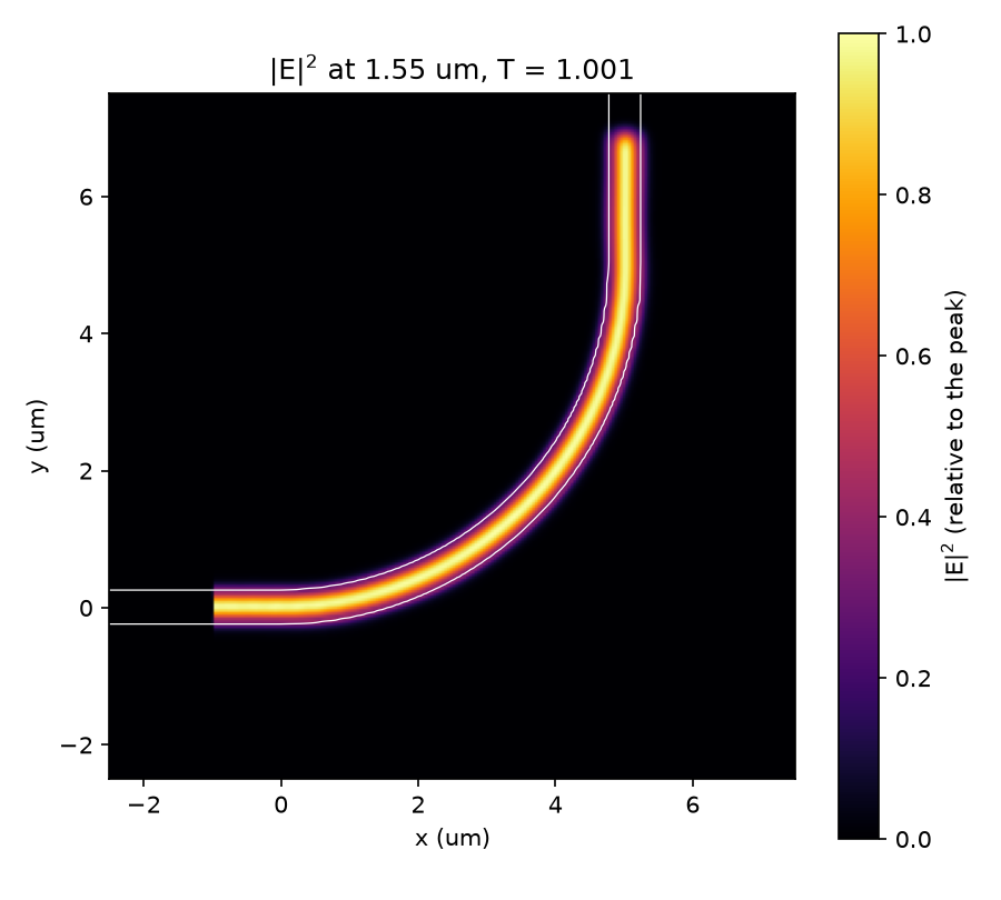
A transmission a little above 1 is not gain: it is the numerical error of the mode amplitudes at this grid, a few parts in a thousand, and it shrinks as the grid is refined (see Choosing the settings). A bend this wide loses less than that error.
How long it takes
About half of the first run is compiling the solver: in one process, the first simulation took 32.7 s and an
identical second one 16.1 s. Without a GPU, try a coarser grid first (--resolution 0.1 took 31 s on 4 CPU cores,
with a transmission of 0.980). The settings are chosen to be quick, not converged.
The script, step by step
1. The component
gf.components.bend_circular, a gdsfactory parametric cell, makes a circular arc with a port at each end: o1 faces
west (orientation 180°) and o2 faces north (90°). The cell and the waveguide layer gf.gpdk.LAYER.WG come from the
generic PDK, which gf.gpdk.PDK.activate() loads. Any other cell, or a component you built yourself, works the same
way. Lengths are in µm.
import argparse
import time
from dataclasses import dataclass
from typing import Any

import fdtdx
import jax
import numpy as np

import gdsfactory as gf
import bifrost as bf
from gdsfactory.technology import LayerLevel, LayerStack

gf.gpdk.PDK.activate()  # the generic PDK: the pcells below and the waveguide layer come from it

WAVELENGTH = 1.55  # um, in vacuum
CORE_INDEX, CLAD_INDEX = 3.48, 1.444  # silicon in silica, constant (no dispersion)
WIDTH, THICKNESS = 0.5, 0.22  # um
RADIUS = 5.0  # um, of the bend's centerline
EXTENSION = 2.5  # um, how far both ports are extended, straight, to the box faces
PML = 1.0  # um of perfectly matched layer inside each face of the box
MARGIN = 2.25  # um of cladding between the bend and the two box faces that have no port
BOX_HEIGHT = 3.4  # um, the box in z; with MARGIN this makes the box exactly 10 x 10 x 3.4 um
PLANE_PADDING = (0.5, 0.3)  # source and monitor planes: wavelengths past the guide, per side (width, height)
RESOLUTION = 0.04  # um, the grid cell
DURATION = 400e-15  # s of simulated time
MOVIE_FRAMES = 40  # time steps the field movie records, evenly spaced

component = gf.components.bend_circular(radius=RADIUS, angle=90, width=WIDTH)  # ports: o1 faces west, o2 north
2. The layer stack and materials
The LayerStack has one level: the core, on the waveguide layer, 0.22 µm thick from z = 0. The materials are
constant-index silicon for the core and silica for the cladding.
LAYER_STACK = LayerStack(
    layers={"core": LayerLevel(layer=gf.gpdk.LAYER.WG, zmin=0.0, thickness=THICKNESS, material="core", mesh_order=1)}
)
MATERIALS = {
    "core": fdtdx.Material(permittivity=CORE_INDEX**2),
    "clad": fdtdx.Material(permittivity=CLAD_INDEX**2),  # also the background
}
3. The device
StackDevice.from_layer_stack voxelizes the component through the stack. background="clad" fills everything the core
does not. extend_ports continues both ports straight out by 2.5 µm, so the guide runs through the absorbing boundary
instead of ending inside the simulation. boundary_offset sets the box: the faces that hold a port stay put, the others
move out by 2.25 µm in x and y, and the box is 3.4 µm tall, 10 × 10 × 3.4 µm in all.
def build_stack() -> bf.StackDevice:
    """The bend voxelized with its layer stack, with both ports extended straight to the box."""
    z_margin = (BOX_HEIGHT - THICKNESS) / 2  # cladding above and below the core
    return bf.StackDevice.from_layer_stack(
        component, LAYER_STACK, MATERIALS,
        background="clad",
        zrange_layers=["core"],    # the box's z range starts as the core's: 0 to 0.22 um
        extend_ports=(("o1", EXTENSION), ("o2", EXTENSION)),  # both end at a box face
        # (x+, x-, y+, y-, z+, z-): the faces holding a port stay put, the others move out. fdtdx rounds
        # the box to whole cells; 10, 10 and 3.4 um are whole numbers of cells at 50, 40, 25 and 20 nm.
        boundary_offset=(MARGIN, 0.0, 0.0, -MARGIN, z_margin, -z_margin),
        name="stack",
    )
Keep the box on the grid
fdtdx rounds each side of the box to a whole number of grid cells when it places it: a 10.03 µm side on a 40 nm grid
becomes 10.04 µm, so the simulated box can differ from boundary_offset by up to half a cell, and changes with the
grid. The script's 10 µm and 3.4 µm are whole numbers of cells at 50, 40, 25 and 20 nm, so the box is the same in
every run of the table below. A side exactly halfway between two cell counts (3.42 µm is
85.5 cells of 40 nm) can make fdtdx stop with Configured grid shape ... does not match simulation volume shape.
4. Wavelength, grid, duration and boundaries
These are fdtdx objects, and fdtdx works in meters: the script's µm lengths are multiplied by 1e-6 where they
enter. SimulationConfig takes the simulated time and the grid, and WaveCharacter the 1.55 µm wavelength. The source
is a pulse 5 % wide in frequency that ramps up smoothly. The absorbing boundary (PML) is 1 µm thick, placed later inside
each face of the box.
    config = stack.get_simulation_config(  # fdtdx.SimulationConfig, in the device's precision (float32 by default)
        time=duration,
        grid=fdtdx.core.grid.UniformGrid(spacing=resolution * 1e-6),
    )
    wave = fdtdx.WaveCharacter(wavelength=WAVELENGTH * 1e-6)
    pulse = fdtdx.GaussianPulseProfile(  # a pulse 5 % wide in frequency, so it ramps up smoothly
        center_wave=wave, spectral_width=fdtdx.WaveCharacter(frequency=0.05 * wave.get_frequency())
    )
    te0 = dict(mode_index=0, filter_pol="te")  # the fundamental TE mode
5. Source and monitors
Everything placed on a port goes through the device. create_mode_plane_source_at launches TE0
(mode_index=0, filter_pol="te") 1 µm outside o1, in the straight extension (a negative port_offset moves a plane
out of the device). create_mode_overlap_detector_at makes monitors of the TE0 that passes a plane: one 0.5 µm outside
o1, counting the mode travelling into the bend, and one 0.5 µm outside o2. Each plane extends 0.5 wavelengths past
the guide's width and 0.3 past its height on each side (PLANE_PADDING). A PhasorDetector records the electric field
at the wavelength on the xy plane through the middle of the core, and a FieldDetector records the same plane at 40
time steps: a movie of the pulse for the viewer.
    volume, constraints = stack.get_simulation_volume()
    objects = [volume, stack]
    for obj, placing in (
        # launch 1 um outside port o1 (a negative port_offset moves a plane out of the device,
        # into the port extension), clear of the absorbing boundary at the box face
        stack.create_mode_plane_source_at(
            "o1", PLANE_PADDING, wave_character=wave, temporal_profile=pulse, port_offset=-1.0,
            name="source", **te0,
        ),
        # one monitor 0.5 um outside each port, in the straight extensions, before and after the bend
        stack.create_mode_overlap_detector_at(
            "o1", PLANE_PADDING, direction="in", wave_characters=(wave,), scaling_mode="pulse",
            port_offset=-0.5, name="in", **te0,
        ),
        stack.create_mode_overlap_detector_at(
            "o2", PLANE_PADDING, wave_characters=(wave,), scaling_mode="pulse",
            port_offset=-0.5, name="out", **te0,
        ),
    ):
        objects.append(obj)
        constraints += placing
    field = fdtdx.PhasorDetector(  # E on the xy plane through the middle of the core
        name="field", wave_characters=(wave,), components=("Ex", "Ey", "Ez"),
        scaling_mode="pulse", partial_grid_shape=(None, None, 1),
    )
    movie = fdtdx.FieldDetector(  # the same plane at 40 evenly spaced time steps: a movie of the pulse
        name="movie", components=("Ex", "Ey"), partial_grid_shape=(None, None, 1),
        switch=fdtdx.OnOffSwitch(interval=max(1, config.time_steps_total // MOVIE_FRAMES)),
    )
    for monitor in (field, movie):
        objects.append(monitor)
        constraints += [monitor.same_size(volume, axes=(0, 1)), monitor.place_at_center(volume)]
    boundaries, placing = fdtdx.boundary_objects_from_config(
        fdtdx.BoundaryConfig.from_uniform_bound(thickness=round(PML / resolution)), volume
    )
    objects += boundaries.values()
    constraints += placing
6. Place, apply and run
fdtdx.place_objects fits everything onto the grid, bf.apply_stack writes the stack into the permittivity (where a
plain fdtdx simulation calls fdtdx.apply_params), and fdtdx.run_fdtd runs the solver.
    key = jax.random.PRNGKey(0)
    objects, arrays, params, config, _ = fdtdx.place_objects(objects, config, constraints, key)
    # write the layer stack into the permittivity arrays (instead of fdtdx.apply_params)
    arrays, objects, _ = bf.apply_stack(arrays, objects, {**params, **bf.init_stack_params(objects)}, key)
    _, arrays = fdtdx.run_fdtd(arrays=arrays, objects=objects, config=config, key=key)
7. Transmission
Each mode monitor stores a complex amplitude: the overlap of TE0 with the plane's field. The input monitor sits in the
straight extension, before the bend has any effect, so it measures what went in; the output monitor measures what came
out. The ratio of their squared magnitudes is the transmission. It is normalized without a reference simulation,
because both monitors use the same mode of the same guide. It counts only light that leaves in TE0 (light scattered into
other modes or the cladding is lost), and not light reflected back, which the input monitor (direction "in") does not
see.
    states = arrays.detector_states
    a_in = objects["in"].compute_overlap(states["in"])  # complex amplitude of TE0 on each monitor
    a_out = objects["out"].compute_overlap(states["out"])
    transmission = float(np.ravel(abs(a_out / a_in) ** 2)[0])  # one entry per wavelength
8. The field image and the viewer
plot_field saves the figure above, with the guide's outline from the permittivity. To explore the result in 3D, load
it into the viewer (in Jupyter or marimo, end the cell with the viewer):
def open_viewer(result: BendResult) -> Any:
    """The viewer with the finished simulation loaded into its Result tab.

    In a Jupyter or marimo cell, end the cell with the returned viewer to display it.
    """
    viewer = bf.view(result.stack)
    viewer.load_result(result.objects, result.arrays, result.config, stack=result.stack)
    return viewer
The viewer opens on the Layout tab; the Result tab shows the field monitors on their planes, the 2D cross-sections and the movie. This exact result, precomputed, is in the live demo.
The complete script
"""A 90 degree silicon waveguide bend, simulated end to end with bifrost and fdtdx.

The device is gdsfactory's ``bend_circular`` pcell. TE0 at 1.55 um is launched into
the straight extension of port ``o1``, and the fraction that leaves port ``o2``
in TE0 is measured. The same script produces the field image
and the result the viewer loads (see docs/getting-started.md).

Run it on a GPU node:  python examples/waveguide_bend.py
Options:               python examples/waveguide_bend.py --resolution 0.04 --figure out.png
"""

import argparse
import time
from dataclasses import dataclass
from typing import Any

import fdtdx
import jax
import numpy as np

import gdsfactory as gf
import bifrost as bf
from gdsfactory.technology import LayerLevel, LayerStack

gf.gpdk.PDK.activate()  # the generic PDK: the pcells below and the waveguide layer come from it

WAVELENGTH = 1.55  # um, in vacuum
CORE_INDEX, CLAD_INDEX = 3.48, 1.444  # silicon in silica, constant (no dispersion)
WIDTH, THICKNESS = 0.5, 0.22  # um
RADIUS = 5.0  # um, of the bend's centerline
EXTENSION = 2.5  # um, how far both ports are extended, straight, to the box faces
PML = 1.0  # um of perfectly matched layer inside each face of the box
MARGIN = 2.25  # um of cladding between the bend and the two box faces that have no port
BOX_HEIGHT = 3.4  # um, the box in z; with MARGIN this makes the box exactly 10 x 10 x 3.4 um
PLANE_PADDING = (0.5, 0.3)  # source and monitor planes: wavelengths past the guide, per side (width, height)
RESOLUTION = 0.04  # um, the grid cell
DURATION = 400e-15  # s of simulated time
MOVIE_FRAMES = 40  # time steps the field movie records, evenly spaced


component = gf.components.bend_circular(radius=RADIUS, angle=90, width=WIDTH)  # ports: o1 faces west, o2 north


LAYER_STACK = LayerStack(
    layers={"core": LayerLevel(layer=gf.gpdk.LAYER.WG, zmin=0.0, thickness=THICKNESS, material="core", mesh_order=1)}
)
MATERIALS = {
    "core": fdtdx.Material(permittivity=CORE_INDEX**2),
    "clad": fdtdx.Material(permittivity=CLAD_INDEX**2),  # also the background
}


def build_stack() -> bf.StackDevice:
    """The bend voxelized with its layer stack, with both ports extended straight to the box."""
    z_margin = (BOX_HEIGHT - THICKNESS) / 2  # cladding above and below the core
    return bf.StackDevice.from_layer_stack(
        component, LAYER_STACK, MATERIALS,
        background="clad",
        zrange_layers=["core"],    # the box's z range starts as the core's: 0 to 0.22 um
        extend_ports=(("o1", EXTENSION), ("o2", EXTENSION)),  # both end at a box face
        # (x+, x-, y+, y-, z+, z-): the faces holding a port stay put, the others move out. fdtdx rounds
        # the box to whole cells; 10, 10 and 3.4 um are whole numbers of cells at 50, 40, 25 and 20 nm.
        boundary_offset=(MARGIN, 0.0, 0.0, -MARGIN, z_margin, -z_margin),
        name="stack",
    )


@dataclass
class BendResult:
    """What a run hands back: the placed simulation (for the viewer) and the numbers."""

    stack: Any
    objects: Any
    arrays: Any
    config: Any
    transmission: float
    field: np.ndarray  # |E|^2 on the xy plane through the middle of the core, shape (nx, ny)
    extent: tuple[float, float, float, float]  # x0, x1, y0, y1 of that plane, um
    eps: np.ndarray  # the permittivity on that plane, shape (nx, ny)
    seconds: float  # wall time of place + apply + run, compilation included
    peak_gib: float | None  # peak device memory, when the backend reports it


def simulate(resolution: float = RESOLUTION, duration: float = DURATION) -> BendResult:
    started = time.perf_counter()
    stack = build_stack()

    config = stack.get_simulation_config(  # fdtdx.SimulationConfig, in the device's precision (float32 by default)
        time=duration,
        grid=fdtdx.core.grid.UniformGrid(spacing=resolution * 1e-6),
    )
    wave = fdtdx.WaveCharacter(wavelength=WAVELENGTH * 1e-6)
    pulse = fdtdx.GaussianPulseProfile(  # a pulse 5 % wide in frequency, so it ramps up smoothly
        center_wave=wave, spectral_width=fdtdx.WaveCharacter(frequency=0.05 * wave.get_frequency())
    )
    te0 = dict(mode_index=0, filter_pol="te")  # the fundamental TE mode

    volume, constraints = stack.get_simulation_volume()
    objects = [volume, stack]
    for obj, placing in (
        # launch 1 um outside port o1 (a negative port_offset moves a plane out of the device,
        # into the port extension), clear of the absorbing boundary at the box face
        stack.create_mode_plane_source_at(
            "o1", PLANE_PADDING, wave_character=wave, temporal_profile=pulse, port_offset=-1.0,
            name="source", **te0,
        ),
        # one monitor 0.5 um outside each port, in the straight extensions, before and after the bend
        stack.create_mode_overlap_detector_at(
            "o1", PLANE_PADDING, direction="in", wave_characters=(wave,), scaling_mode="pulse",
            port_offset=-0.5, name="in", **te0,
        ),
        stack.create_mode_overlap_detector_at(
            "o2", PLANE_PADDING, wave_characters=(wave,), scaling_mode="pulse",
            port_offset=-0.5, name="out", **te0,
        ),
    ):
        objects.append(obj)
        constraints += placing
    field = fdtdx.PhasorDetector(  # E on the xy plane through the middle of the core
        name="field", wave_characters=(wave,), components=("Ex", "Ey", "Ez"),
        scaling_mode="pulse", partial_grid_shape=(None, None, 1),
    )
    movie = fdtdx.FieldDetector(  # the same plane at 40 evenly spaced time steps: a movie of the pulse
        name="movie", components=("Ex", "Ey"), partial_grid_shape=(None, None, 1),
        switch=fdtdx.OnOffSwitch(interval=max(1, config.time_steps_total // MOVIE_FRAMES)),
    )
    for monitor in (field, movie):
        objects.append(monitor)
        constraints += [monitor.same_size(volume, axes=(0, 1)), monitor.place_at_center(volume)]
    boundaries, placing = fdtdx.boundary_objects_from_config(
        fdtdx.BoundaryConfig.from_uniform_bound(thickness=round(PML / resolution)), volume
    )
    objects += boundaries.values()
    constraints += placing

    key = jax.random.PRNGKey(0)
    objects, arrays, params, config, _ = fdtdx.place_objects(objects, config, constraints, key)
    # write the layer stack into the permittivity arrays (instead of fdtdx.apply_params)
    arrays, objects, _ = bf.apply_stack(arrays, objects, {**params, **bf.init_stack_params(objects)}, key)
    _, arrays = fdtdx.run_fdtd(arrays=arrays, objects=objects, config=config, key=key)

    states = arrays.detector_states
    a_in = objects["in"].compute_overlap(states["in"])  # complex amplitude of TE0 on each monitor
    a_out = objects["out"].compute_overlap(states["out"])
    transmission = float(np.ravel(abs(a_out / a_in) ** 2)[0])  # one entry per wavelength

    k = objects["field"].grid_slice[2].start  # z index of the field plane
    phasor = np.asarray(states["field"]["phasor"][0, 0, :, :, :, 0])  # (3, nx, ny) at the wavelength
    nx, ny = phasor.shape[1:]
    sx, sy, _ = (float(v) * 1e6 for v in stack.partial_real_shape)
    x0, y0 = float(stack.center[0]) - sx / 2, float(stack.center[1]) - sy / 2
    stats = getattr(jax.devices()[0], "memory_stats", lambda: None)()
    return BendResult(
        stack=stack, objects=objects, arrays=arrays, config=config, transmission=transmission,
        field=np.sum(np.abs(phasor) ** 2, axis=0),
        extent=(x0, x0 + nx * resolution, y0, y0 + ny * resolution),
        eps=1 / np.asarray(arrays.inv_permittivities[0, :, :, k]),
        seconds=time.perf_counter() - started,
        peak_gib=None if not stats else stats.get("peak_bytes_in_use", 0) / 2**30,
    )


def open_viewer(result: BendResult) -> Any:
    """The viewer with the finished simulation loaded into its Result tab.

    In a Jupyter or marimo cell, end the cell with the returned viewer to display it.
    """
    viewer = bf.view(result.stack)
    viewer.load_result(result.objects, result.arrays, result.config, stack=result.stack)
    return viewer


def plot_field(result: BendResult, path: str) -> None:
    """Saves |E|^2 on the xy plane through the core, with the guide's outline."""
    import matplotlib

    matplotlib.use("Agg")
    import matplotlib.pyplot as plt

    x0, x1, y0, y1 = result.extent
    fig, ax = plt.subplots(figsize=(6, 5.4))
    image = ax.imshow(
        result.field.T / result.field.max(), origin="lower", extent=(x0, x1, y0, y1), cmap="inferno",
    )
    xs, ys = np.linspace(x0, x1, result.eps.shape[0]), np.linspace(y0, y1, result.eps.shape[1])
    ax.contour(xs, ys, result.eps.T, levels=[(CORE_INDEX**2 + CLAD_INDEX**2) / 2], colors="white", linewidths=0.6)
    ax.set(xlabel="x (um)", ylabel="y (um)", title=f"|E|$^2$ at {WAVELENGTH} um, T = {result.transmission:.3f}")
    fig.colorbar(image, label="|E|$^2$ (relative to the peak)")
    fig.tight_layout()
    fig.savefig(path, dpi=150)


if __name__ == "__main__":
    parser = argparse.ArgumentParser(description=__doc__.splitlines()[0])
    parser.add_argument("--resolution", type=float, default=RESOLUTION, help="grid cell in um")
    parser.add_argument("--duration", type=float, default=DURATION, help="simulated time in s")
    parser.add_argument("--figure", default="waveguide_bend_field.png", help="where to save the field image")
    args = parser.parse_args()

    result = simulate(args.resolution, args.duration)
    print(f"transmission: {result.transmission:.4f}")
    print(f"wall time:    {result.seconds:.1f} s (compilation included)")
    if result.peak_gib is not None:
        print(f"peak memory:  {result.peak_gib:.1f} GiB on {jax.devices()[0]}")
    plot_field(result, args.figure)
    print(f"field image:  {args.figure}")
Choosing the settings
The same script on an NVIDIA L40S at four grids, each in its own process (scripts/bend_sweep.py reproduces the table).
The transmission moves by less than 0.2 %, so the script uses 40 nm; a more sensitive device would need a finer grid.
| Grid cell | Transmission | Wall time | Peak GPU memory |
|---|---|---|---|
| 50 nm | 1.0012 | 24 s | 0.7 GiB |
| 40 nm (the script's default) | 1.0008 | 32 s | 1.2 GiB |
| 25 nm | 0.9998 | 106 s | 4.6 GiB |
| 20 nm | 0.9994 | 227 s | 8.7 GiB |
A run 1.5 times as long (600 fs) gives the same transmission to four digits at 25 nm (0.9998), so 400 fs is enough for the pulse to cross the device and ring down.
Troubleshooting
- The run takes forever, or
jax.devices()shows only a CPU. JAX found no accelerator: see JAX setup. On a CPU, coarsen the grid (--resolution 0.1) to try the script. - The first run is slow but later ones are fast. The first call compiles the solver for this grid size. Changing the box or the grid compiles again.
RESOURCE_EXHAUSTEDor an out-of-memory error. The grid is too fine for the accelerator's memory, which grows with the cube of the refinement (see the table). Use a coarser--resolutionor a smaller box.Configured grid shape ... does not match simulation volume shape. A side of the box is exactly halfway between two cell counts, and fdtdx rounded it differently in two places. Moveboundary_offsetby a fraction of a cell, or change the grid spacing; see step 3.- The viewer shows nothing in a plain script. The viewer is a notebook widget: run the code in Jupyter or marimo and end the cell with the viewer, or look at the live demo.
- The transmission is 0 or absurd. Check the units (fdtdx wants meters:
1e-6), that the source is not inside the PML, and that each plane lies inside the box. See Simulation setup and ports.
Next
- Simulation setup and ports: sources, monitors and the run, in detail.
- Results and field monitors: reading what the monitors record.
- Gradients: differentiate a result with respect to the geometry, through the simulation.
- Inverse design: optimize the width profile of a tight bend for transmission.