Inverse design¶

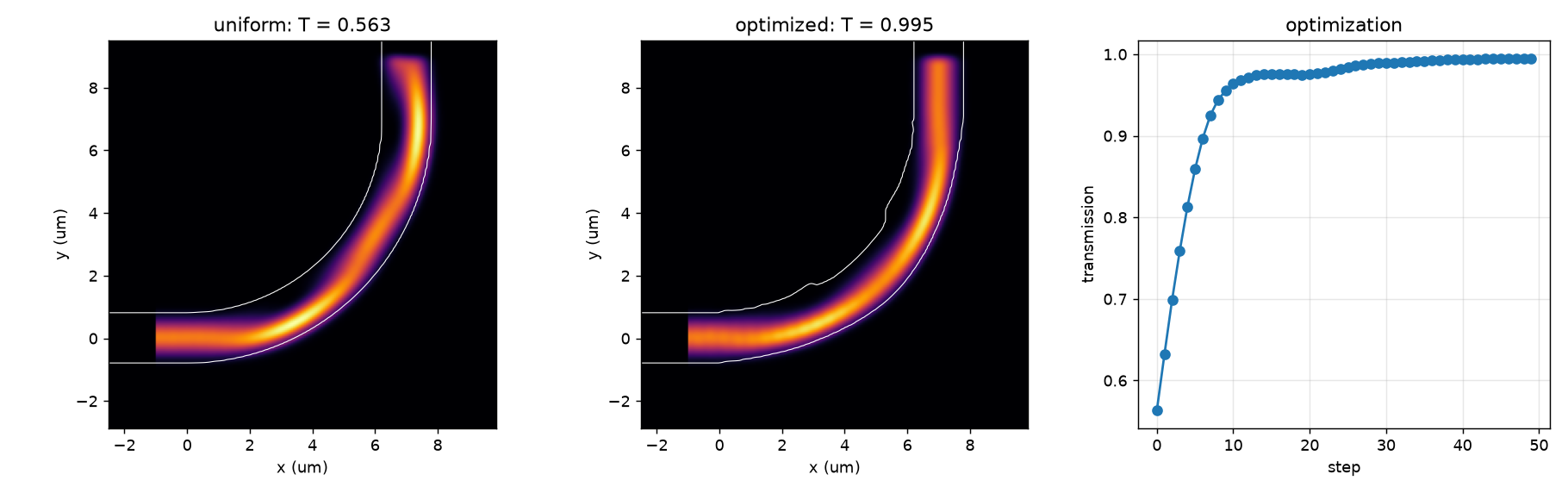
An air-clad silicon nitride guide on silica, 1.6 µm wide and 0.75 µm thick, bent 90° at 7 µm radius, transmits only 56 % of TE0 at 1.55 µm as TE0 at its uniform width: most of the rest leaves the bend as TE1. examples/guide/inverse_design.py optimizes the width on each side of its centerline, at 70 stations, for TE0 transmission, by gradient ascent through the simulation, and raises it to 99.5 %: the bend's loss falls from 2.5 dB to 0.02 dB, and a finer grid confirms it. Run it on a GPU; on an NVIDIA L40S its 50 steps took 3146 s.

The uniform and the optimized bend: |E|² on the middle of the core, and the transmission per step

The bend and its parameters¶

WAVELENGTH = 1.55  # um
CORE_INDEX, BOX_INDEX, CLAD_INDEX = 1.996, 1.444, 1.0  # silicon nitride on silica, under air
WIDTH, THICKNESS = 1.6, 0.75  # um: the guide at both ports
RADIUS = 7.0  # um, of the bend's centerline
N_STATIONS = 70  # evenly spaced along the bend between its two ends
H_MIN, H_MAX = 0.25, 1.25  # um: bounds of every half-width (H_MAX < RADIUS keeps the inner edge off the center)
ANGLES = jnp.linspace(0.0, jnp.pi / 2, N_STATIONS + 2)  # one vertex per station and end on each edge: a fixed topology


def tight_bend(half_widths):
    """The bend whose inner and outer edges are ``half_widths`` (2, N_STATIONS) um from its centerline.

    Row 0 is the side toward the bend's center, row 1 the side away from it. At both ends the guide is
    WIDTH wide and centered; in between, each edge is linear from station to station. Every profile has
    the same 144 vertices, so the device built for one takes the vertices of any other (``StackDevice.pack``).
    """
    t = ANGLES / ANGLES[-1]  # along the bend, 0 to 1
    stations = jnp.linspace(0.0, 1.0, N_STATIONS + 2)
    end = jnp.array([WIDTH / 2])
    h_in, h_out = (jnp.interp(t, stations, jnp.concatenate([end, h, end])) for h in jnp.asarray(half_widths))
    edges = []
    for r in (RADIUS + h_out, RADIUS - h_in):  # the arc's center is at (0, RADIUS)
        edges.append(jnp.stack([r * jnp.sin(ANGLES), RADIUS - r * jnp.cos(ANGLES)], axis=1))
    bend = gf.Component()
    bend.add_polygon(jnp.concatenate([edges[0], edges[1][::-1]]), layer=gf.gpdk.LAYER.WG)
    bend.add_port(name="o1", center=(0.0, 0.0), width=WIDTH, orientation=180, layer=gf.gpdk.LAYER.WG)
    bend.add_port(name="o2", center=(RADIUS, RADIUS), width=WIDTH, orientation=90, layer=gf.gpdk.LAYER.WG)
    return bend


UNIFORM = jnp.full((2, N_STATIONS), WIDTH / 2)  # the 1.6 um guide, centered everywhere

The guide: 1.6 µm wide and 0.75 µm thick, it guides four modes: TE0 (effective index 1.81), TM0 (1.76), TE1 (1.63) and TM1 (1.61); TE2 (1.436) is below the silica's 1.444.
Where the light goes: the uniform bend transmits 0.563 of TE0 as TE0 and 0.405 as TE1 (on the 60 nm grid; 0.559 and 0.414 at 40 nm). Nearly all the light gets through, but 41 % of the input leaves as TE1: the straight guide's mode does not match the bend's, which sits toward its outer edge, so the junctions excite both bend modes. Only 3 % is lost otherwise.
Both ends are fixed: 1.6 µm wide and centered, so the ports, their straight leads and the monitors in them never change. Only the 70 stations in between move, each edge linear from one to the next.
The topology is fixed: every profile has the same 144 vertices, one per station and end on each edge, so the device built once, for the uniform bend, takes any profile's vertices with stack.pack (see polygon topology).
Two widths per station, toward the bend's center and away from it. A single width, symmetric about the centerline, helps here: narrowing the bend to 1.2 µm raises the transmission to 0.85 (widening it to 2.0 µm lowers it to 0.25). Moving the guide toward the center, so the straight guide's mode lines up with the bend's, helps more: 0.1, 0.2 and 0.3 µm give 0.82, 0.96 and 0.92. Only two independent edges can express both.

The simulation¶

As in Gradients, with the source 1 µm and both monitors 0.5 µm out in the straight leads, clear of the moving edges: a monitor on the port itself would see the bend's edges move and change the mode it measures. The silica is a level on the WAFER layer that runs through the bottom of the box, under an air background (see Adding a substrate). The mode reaches into the silica, so the box is 4.8 µm tall and the source and monitor planes reach 0.5 wavelengths (0.78 µm) above and below the core, where the mode's field has fallen to about 3 %, still clear of the absorbing layers.

EXTENSION = 2.5  # um: both ports run straight out to the box faces
MARGIN = 2.06  # um past the bend's two free sides; the box is 12.36 x 12.36 x 4.8 um, whole cells at 60 and 40 nm
BOX_HEIGHT, PML = 4.8, 1.0  # um
RESOLUTION, CHECK_RESOLUTION = 0.06, 0.04  # um: the grid it is optimized on, and the finer one it is checked on
DURATION = 500e-15  # s
PADDING = (0.5, 0.5)  # wavelengths past the port's width and the core's height: the mode reaches into the silica
KEY = jax.random.PRNGKey(0)

layer_stack = LayerStack(
    layers={
        "box": LayerLevel(layer="WAFER", zmin=-3.0, thickness=3.0, material="silica", mesh_order=9),
        "core": LayerLevel(layer=gf.gpdk.LAYER.WG, zmin=0.0, thickness=THICKNESS, material="core", mesh_order=1),
    }
)
materials = {
    "core": fdtdx.Material(permittivity=CORE_INDEX**2),
    "silica": fdtdx.Material(permittivity=BOX_INDEX**2),
    "air": fdtdx.Material(permittivity=CLAD_INDEX**2),
}


def place(resolution):
    """The uniform bend, placed on a grid of this cell (um) with its source and monitors."""
    z_margin = (BOX_HEIGHT - THICKNESS) / 2  # the silica runs through the bottom face, the air through the top
    stack = bf.StackDevice.from_layer_stack(
        tight_bend(UNIFORM), layer_stack, materials, background="air", zrange_layers=["core"],
        extend_ports=(("o1", EXTENSION), ("o2", EXTENSION)),
        boundary_offset=(MARGIN, 0, 0, -MARGIN, z_margin, -z_margin), name="stack",
    )
    config = stack.get_simulation_config(
        time=DURATION, grid=fdtdx.core.grid.UniformGrid(spacing=resolution * 1e-6),
        gradient_config=fdtdx.GradientConfig(method="checkpointed", num_checkpoints=60),  # bounded backward memory
    )
    wave = fdtdx.WaveCharacter(wavelength=WAVELENGTH * 1e-6)
    pulse = fdtdx.GaussianPulseProfile(
        center_wave=wave, spectral_width=fdtdx.WaveCharacter(frequency=0.05 * wave.get_frequency())
    )
    te0 = dict(mode_index=0, filter_pol="te")
    volume, constraints = stack.get_simulation_volume()
    objects = [volume, stack]
    for obj, placing in (
        # source and monitors in the straight leads, clear of the bend whose edges move
        stack.create_mode_plane_source_at(
            "o1", PADDING, wave_character=wave, temporal_profile=pulse, port_offset=-1.0, name="source", **te0,
        ),
        stack.create_mode_overlap_detector_at(
            "o1", PADDING, direction="in", wave_characters=(wave,), scaling_mode="pulse", port_offset=-0.5,
            name="in", **te0,
        ),
        stack.create_mode_overlap_detector_at(
            "o2", PADDING, wave_characters=(wave,), scaling_mode="pulse", port_offset=-0.5, name="out", **te0,
        ),
    ):
        objects.append(obj)
        constraints += placing
    field = fdtdx.PhasorDetector(  # E on the xy plane through the middle of the core, for the figure
        name="field", wave_characters=(wave,), components=("Ex", "Ey", "Ez"), scaling_mode="pulse",
        partial_grid_shape=(None, None, 1),
    )
    objects.append(field)
    constraints += [field.same_size(volume, axes=(0, 1)), field.place_at_center(volume)]
    boundaries, placing = fdtdx.boundary_objects_from_config(
        fdtdx.BoundaryConfig.from_uniform_bound(thickness=round(PML / resolution)), volume
    )
    objects += boundaries.values()
    constraints += placing
    objects, arrays, params, config, _ = fdtdx.place_objects(objects, config, constraints, KEY)
    return objects, arrays, {**params, **bf.init_stack_params(objects)}, config

Objective and optimizer¶

The objective is the normalized TE0 transmission |a_out / a_in|². Each half-width is a bounded function of an unbounded parameter, so the optimizer cannot leave 0.25 to 1.25 µm (a guide 0.5 to 2.5 µm wide), and optax's Adam (installed with fdtdx) steps on those parameters. jax.value_and_grad of the objective is wrapped in bf.jit, so the cell function, apply_stack, the simulation and its backward pass compile into one program, once, at the first step: every step has the same shapes, and the cell function's structure (144 vertices, no branch on a half-width) does not depend on the parameters, so gdsfactoryx can trace it (see the gdsfactoryx README). The arrays and parameters are arguments of the compiled function rather than constants captured by the trace.

bf.jit is jax.jit with one XLA option: with plain jax.jit, XLA turns the conditional in the backward loop of fdtdx's checkpointed time loop into a select, and computes a time step's VJP on every iteration of that loop, recomputations of forward steps included. Here the example took 4848 s with jax.jit and 3146 s with bf.jit, with the same results (see bf.jit).

def simulate(half_widths, placed):
    """Transmission (TE0 power out over TE0 power in) of the bend with these half-widths, and the final arrays."""
    objects, arrays, params, config = placed
    stack = objects["stack"]
    p = {**params, "stack": {**params["stack"], **stack.pack(tight_bend(half_widths))}}  # the new edges' vertices
    arrays, objects, _ = bf.apply_stack(arrays, objects, p, KEY)
    _, arrays = fdtdx.run_fdtd(arrays=arrays, objects=objects, config=config, key=KEY, show_progress=False)
    a_in = objects["in"].compute_overlap(arrays.detector_states["in"])
    a_out = objects["out"].compute_overlap(arrays.detector_states["out"])
    return jnp.abs(a_out / a_in)[0] ** 2, arrays


def half_widths_of(z):
    """Unbounded parameters to half-widths within (H_MIN, H_MAX): the optimizer never leaves the bounds."""
    return H_MIN + (H_MAX - H_MIN) * jax.nn.sigmoid(z)


def parameters_of(half_widths):
    """The inverse of half_widths_of."""
    u = (jnp.asarray(half_widths) - H_MIN) / (H_MAX - H_MIN)
    return jnp.log(u / (1 - u))

def describe(half_widths):
    """The range of a profile's width, and of its middle's shift toward the bend's center (um)."""
    inner, outer = np.asarray(half_widths)
    width, shift = inner + outer, (inner - outer) / 2
    return f"width {width.min():.2f} to {width.max():.2f}, shift {shift.min():+.2f} to {shift.max():+.2f} um"


def optimize(placed, iterations, learning_rate=0.03):
    """Adam on the transmission; returns the best half-widths seen and the transmission of every step."""
    objects, arrays, params, config = placed

    def objective(z, arrays, params):
        return simulate(half_widths_of(z), (objects, arrays, params, config))[0]

    # compiled once, at the first step: every step has the same shapes. bf.jit is jax.jit with an XLA option that
    # keeps the backward pass from computing a time step's VJP on every iteration, recomputations included
    # (see bifrost.jitting)
    value_and_grad = bf.jit(jax.value_and_grad(objective))
    optimizer = optax.adam(learning_rate)
    # start from the uniform bend, float64 and committed to the device like the optimizer's updates (a weakly typed
    # or uncommitted start would compile the step twice)
    z = jax.device_put(jnp.asarray(parameters_of(UNIFORM), dtype=jnp.float64), jax.devices()[0])
    state = optimizer.init(z)
    history, best = [], (-1.0, None)
    for step in range(iterations):
        transmission, gradient = value_and_grad(z, arrays, params)
        transmission = float(transmission)
        history.append(transmission)
        print(f"step {step:2d}  T = {transmission:.4f}  {describe(half_widths_of(z))}")
        if transmission > best[0]:
            best = (transmission, half_widths_of(z))
        updates, state = optimizer.update(-gradient, state)  # optax minimizes: ascend on T
        z = optax.apply_updates(z, updates)
    return best[1], history

Result¶

    placed = place(args.resolution)
    half_widths, history = optimize(placed, args.iterations)
    print(f"optimized: {describe(half_widths)}")
    images = {name: field_image(h, placed, args.resolution) for name, h in (("uniform", UNIFORM), ("optimized", half_widths))}
    t_uniform, t_optimized = images["uniform"][0], images["optimized"][0]
    print(f"transmission at {args.resolution * 1e3:.0f} nm: uniform {t_uniform:.4f}, optimized {t_optimized:.4f}")
    if args.check:
        fine = place(args.check)  # the same two designs on a finer grid: is the gain real?
        t_uniform, t_optimized = (float(simulate(h, fine)[0]) for h in (UNIFORM, half_widths))
        print(f"transmission at {args.check * 1e3:.0f} nm: uniform {t_uniform:.4f}, optimized {t_optimized:.4f}")

Output (steps 2 to 4, 6 to 9, 11 to 14, 16 to 19, 21 to 29 and 31 to 48 left out):

step  0  T = 0.5634  width 1.60 to 1.60, shift +0.00 to +0.00 um
step  1  T = 0.6326  width 1.59 to 1.60, shift -0.01 to +0.01 um
step  5  T = 0.8591  width 1.53 to 1.60, shift -0.04 to +0.04 um
step 10  T = 0.9636  width 1.47 to 1.61, shift -0.07 to +0.07 um
step 15  T = 0.9760  width 1.44 to 1.65, shift -0.08 to +0.09 um
step 20  T = 0.9756  width 1.45 to 1.68, shift -0.09 to +0.11 um
step 30  T = 0.9894  width 1.54 to 1.74, shift -0.07 to +0.11 um
step 49  T = 0.9950  width 1.52 to 1.75, shift -0.07 to +0.12 um
optimized: width 1.52 to 1.75, shift -0.07 to +0.12 um
transmission at 60 nm: uniform 0.5634, optimized 0.9950
transmission at 40 nm: uniform 0.5586, optimized 0.9934
wall time: 3146 s on NVIDIA L40S

The design: the guide stays 1.52 to 1.75 µm wide, and its middle moves by up to 0.12 µm toward the center and 0.07 µm away from it along the bend. In the figure, the uniform bend's field beats across the guide as TE0 and TE1 interfere; the optimized bend carries one mode along its outer edge. With no penalty on curvature, the inner edge, where little light goes, keeps ripples a few stations long; a design for fabrication would smooth or penalize them.
The best step is kept: here it is the last, but the transmission dips slightly at steps 17 to 19. With a learning rate of 0.1 instead of 0.03 it reaches 0.954 at step 3, falls to 0.928 by step 7 and recovers, so optimize returns the best widths it has seen, not the last. That run ends at a similar transmission (0.9962; 0.9940 at 40 nm), with the guide up to 1.96 µm wide and a rougher inner edge.
The gain is the device's, not the grid's: on the 40 nm grid the uniform bend transmits 0.5586 and the optimized one 0.9934. The derivatives are those of the discretized simulation (see what the derivatives are), so an optimum is worth checking on a finer grid.
The time: 50 steps, each a forward and a backward solve, then four forward solves for the figure and the check.

For your own designs¶

Choose parameters that can express the improvement: here, two edges rather than one symmetric width.
Scale the step to the parameters: with 140 of them, Adam's early steps move every edge by about the same amount, so a smaller learning rate gives a steadier rise and a smoother profile.
Bound them through a smooth map (here a sigmoid) instead of clipping, which would stop their gradients at the bounds.
Keep the ports and the leads that hold the monitors fixed, and keep the number of vertices fixed; for a change of topology, rebuild the device with retopologize (see polygon topology).
Keep the best design seen, and check it on a finer grid.